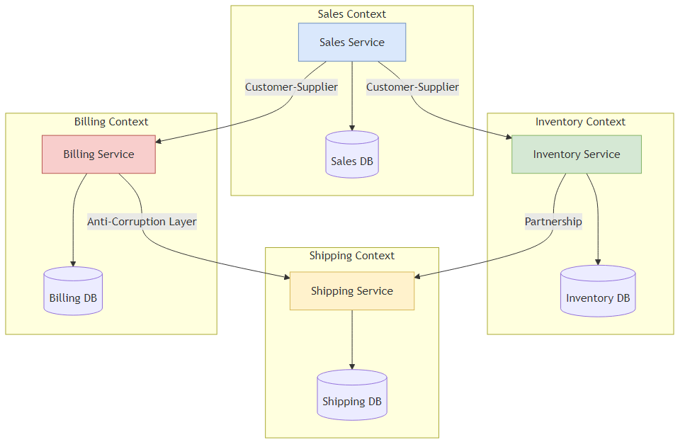
 Figure 3.2: Context map showing relationships between bounded contexts with different coupling patterns and power dynamics
“Total unification of the domain model for a large system won’t be feasible or cost effective.”
— Eric Evans, Domain Driven Design
If Conway’s Law (Chapter 2) describes the human topology of a system, Domain Driven Design (DDD) describes its semantic topology.
For the Senior Architect, DDD is often misunderstood. it’s frequently conflated with its “Tactical” patterns Entities, Value Objects, Repositories, and Aggregates. While these patterns are vital for
Writing clean code within a service, they don’t solve the distributed system problem. You can build a perfectly valid “Aggregate” and still create a Distributed Monolith if that Aggregate is the wrong size or coupled to the wrong things.
The Architect’s primary concern is Strategic Design: determining where the model stops being valid. The single biggest cause of microservice failure is the attempt to create a “Single Source of Truth” for complex concepts like “Customer” or “Product” across the entire enterprise. This creates a Semantic Lock—a rigid dependency where every team must agree on a single definition, paralyzing velocity.
To decouple the system, we must first decouple the language.
In monolithic architecture, we strive for unification. We want one User table, one Product class, and one Order service. We normalize data to eliminate redundancy.
In distributed architecture, this goal is an anti-pattern.
In linguistics, polysemy is the capacity for a word to have multiple related meanings. In enterprise software, polysemy is the enemy of decoupling.
Consider the concept of a “Book” in a large publishing house:
Editorial Context: A “Book” is a manuscript. It has drafts, edits, a word count, and an author relationship. It doesn’t have a price or dimensions yet.
Printing/Logistics Context: A “Book” is a physical object. It has dimensions (H × W × D), paper weight, binding type, and warehouse location. It doesn’t care about the plot or the author.
eCommerce/Sales Context: A “Book” is a product SKU. It has a price, a star rating, a cover image, and shipping eligibility.
Legal/Rights Context: A “Book” is an intellectual property asset with territories, royalty percentages, and expiration dates.
The Monolithic Mistake:
The novice architect attempts to create a single Book entity that satisfies all these needs.
1
2
3
4
5
6
7
8
9
10
11
12
// The "God Class" Anti-Pattern
public class Book {
    private String isbn;
    private String title;          // Editorial
    private String authorId;       // Editorial
    private double weightKg;       // Logistics
    private String warehouseBin;   // Logistics
    private BigDecimal price;      // Sales
    private double royaltyRate;    // Legal
    private List<Contract> rights; // Legal
    //... 50 more fields...
}
This class becomes a dependency magnet. If the Logistics team needs to change how they track warehouse bins, they must modify the Book class, potentially breaking the Editorial system. The Book service becomes a bottleneck where all requirements converge. I’ve seen this pattern destroy velocity in multiple organizations.
The Distributed Solution (Bounded Contexts):
We accept that “Book” means different things in different contexts. We create distinct models for each.
These models are linked only by an ID (e.g., ISBN). They share nothing else. This is the Bounded Context: the specific boundary within which a model applies.
A common point of confusion is the distinction between Subdomains and Bounded Contexts.
The Problem Space (Subdomains):
This is the reality of the business. It exists whether you write software or not.
The Solution Space (Bounded Contexts):
This is the software you write.
The Strategic Mapping:
Ideally, one Bounded Context maps to one Subdomain.
Success Scenario: The “Recommendation Engine” (Core Domain) is its own microservice (Bounded Context). The team works exclusively on algorithms.
Failure Scenario: The “Recommendation Engine” is mixed into the “Catalog Service” (Supporting Subdomain). The algorithms team can’t deploy because the Catalog team is fixing a CRUD bug.
Invest your best talent in the Core Domain. Buy or outsource Generic Subdomains. don’t build your own Identity Provider unless you are Okta. don’t build your own Ledger unless you are a bank.
3.2 Context Mapping: The Politics of Code
Once you have identified your contexts (and potential microservices), you must define how they interact. This is Context Mapping. it’s as much a political activity as a technical one, as it describes the power dynamics between teams.
Static architecture diagrams (boxes and arrows) lie. They imply that all connections are equal. In reality, the relationship between “Billing” and “Sales” is very different from the relationship between “Sales” and “Mainframe Legacy.”
3.2.1 The Seven Relationships
The Senior Architect uses these patterns to categorize dependencies and calculate the “coupling tax.”
| Pattern | Definition | Power Dynamic | Coupling Risk |
|---|---|---|---|
| Partnership | Two teams work together on two contexts that succeed or fail together. | Cooperative. High bandwidth communication required. | High. Synchronization of deployment is often required. Avoid this for long-term stability. |
| Shared Kernel | Two teams share a subset of the model (e.g., a shared JAR library). | Cooperative. “If you change it, you break me.” | Extreme. Changes to the kernel require consensus. Keep the kernel tiny (e.g., basic types like Money, CountryCode). |
| Customer-Supplier | Upstream (Supplier) provides a service to Downstream (Customer). Suppliers can veto changes. | Upstream Dominance. Supplier dictates the schedule. | Medium. Downstream is dependent on Upstream’s roadmap. |
| Conformist | Downstream has no influence over Upstream. Example: Integrating with Amazon API or a massive Legacy ERP. | Dictatorship. “Take it or leave it.” | High. Downstream models are polluted by Upstream concepts. |
| Anti-Corruption Layer (ACL) | Downstream builds a translation layer to isolate itself from Upstream. | Defensive. Downstream protects its purity. | Low. Decouples the domain models at the cost of complexity. |
| Open Host Service (OHS) | Upstream provides a standardized, public API for many consumers. | Service Provider. Upstream commits to backward compatibility. | Low. Standard REST/gRPC contracts with strict versioning. |
| Published Language | A standard interchange format (e.g., iCal, XML standards) used by both. | Standardized. Neither side owns the format. | Low. Very loose coupling. |
3.2.2 The Context Map Visualization
The Architect must maintain a live Context Map. Unlike a UML diagram, this map includes the quality of the connection.
Figure 3.2: Context map showing relationships between bounded contexts with different coupling patterns and power dynamics
Analysis: The Recommendation Service “Conforms” to Identity (it just uses the UserID provided). However, it uses an ACL to talk to the Mainframe. Why? Because the Mainframe uses obscure COBOL data structures that we don’t want leaking into our modern Python recommendation algorithms.
3.3 The Anti-Corruption Layer (ACL): The Migration Bridge
The Anti-Corruption Layer is the most critical pattern for modernizing legacy systems. It allows you to build a new, clean microservice that interacts with a “Big Ball of Mud” monolith without becoming infected by the monolith’s bad design.
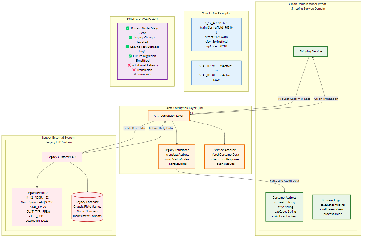 Figure 3.1: Anti-Corruption Layer pattern protecting clean domain models from legacy system complexity through translation and adaptation layers
The ACL consists of three components:
Scenario: A new ShippingService needs address data from a 30-year-old LegacyERP. The ERP stores addresses in a single pipe-delimited string column called K_12_ADDR and uses 99 for “Active” users.
The Goal: The ShippingService domain model should have a clean Address object and a boolean isActive. It should never see K_12_ADDR.
1
2
3
4
5
6
7
8
9
10
11
12
13
14
15
16
17
18
19
20
21
22
23
24
25
26
27
28
29
30
31
32
33
34
35
36
37
38
39
40
41
42
43
44
45
46
47
48
49
50

// 1. The Domain Model (Clean    What we want)
package com.shipping.domain;

public record CustomerAddress(
    String street,
    String city,
    String zipCode,
    boolean isActive
) {}

// 2. The Legacy Data Structure (Dirty    What we get)
package com.shipping.infrastructure.legacy;

public class LegacyUserDTO {
    public String K_12_ADDR; // "123 Main St|Springfield|90210"
    public int STAT_ID;      // 99 = Active, 00 = Deleted
}

// 3. The Translator (The Logic)
@Component
public class LegacyTranslator {
    public CustomerAddress translate(LegacyUserDTO dirty) {
        if (dirty == null) return null;

// Decrypt the legacy pipe  delimited madness
        String parts = dirty.K_12_ADDR.split("\\|");
        String street = parts.length > 0? parts : "";
        String city   = parts.length > 1? parts[1] : "";
        String zip    = parts.length > 2? parts[2] : "";

// Map Magic Numbers to Boolean
        boolean active = (dirty.STAT_ID == 99);

return new CustomerAddress(street, city, zip, active);
    }
}

// 4. The Facade / Service Adapter (The Gatekeeper)
@Service
public class CustomerProfileAdapter implements CustomerProfilePort {
    private final LegacyClient legacyClient;
    private final LegacyTranslator translator;

public CustomerAddress getProfile(String customerId) {
        LegacyUserDTO rawData = legacyClient.fetchUser(customerId);
        // The ACL ensures rawData never escapes this method
        return translator.translate(rawData);
    }
}
Pro: The ShippingService core logic is pristine. If the Legacy ERP changes K_12_ADDR to comma delimited, you only change the LegacyTranslator. The domain logic remains untouched.
Con: Latency. You are adding an object allocation and string parsing step to every call. Maintenance. You now own a translation layer that must be kept in sync.
Problem: How do you find the correct Bounded Contexts in the first place?
Invented by Alberto Brandolini, this is a workshop format for rapidly exploring complex business domains. it’s the antidote to “Analysis Paralysis.”
It is not a “meeting.” it’s a massive, visual collaborative modeling session.
The Room: You need a wall. A really big wall (at least 5 meters). Remove all chairs. People must stand.
The Participants: You need the “Questions” (Developers) and the “Answers” (Domain Experts/Business Stakeholders). If the Domain Experts are not there, cancel the session.
Materials: Sticky notes in specific colors.
Time: 20 Minutes.
Instruction: “Write down every event that happens in the system on an Orange sticky note. Use Past Tense (e.g., OrderPlaced, PaymentFailed, ItemShipped). don’t organize them yet.”
Goal: Quantity over quality. Get the domain knowledge out of people’s heads and onto the wall.
Time: 30-45 Minutes.
Instruction: “Arrange the events chronologically from left to right.”
Observation: Arguments will start. “Does InventoryReserved happen before or after PaymentAuthorized?”
Architect’s Note: These arguments are the gold. They reveal ambiguity. Mark these spots with a bright red “Hot Spot” sticky note to revisit later.
Time: 40 Minutes.
Instruction: “What caused this event?”
Action: Add Blue stickies (Commands) before the events. Add Yellow stickies (Actors) who invoked the command.
Flow: User (Yellow) → Place Order (Blue) → OrderCreated (Orange).
This is the most critical step for microservice boundaries.
The Architect’s Eye: Look for the same noun appearing in distant clusters.
In the Sales cluster, we see LeadConverted and ContractSigned. The “Customer” here is a prospect.
In the Fulfillment cluster, we see PackageShipped. The “Customer” here is a shipping address.
The Heuristic: Identify the Pivotal Events where the meaning changes.
When OrderConfirmed happens, the meaning of the data changes from “Shopping Cart” (volatile, marketing heavy) to “Shipment” (immutable, logistics heavy).
Draw a line here. This is a candidate Bounded Context boundary.
Instruction: “Draw circles around clusters of events that share the same language and data consistency requirements.”
Circle 1: “Sales Context” (Handles leads, opportunities).
Circle 2: “Fulfillment Context” (Handles picking, packing, shipping).
Interaction: They communicate only via the OrderConfirmed domain event.
Don’t just take photos. Convert the circles into Aggregates and Services.
Sales Context becomes the Sales Microservice.
Fulfillment Context becomes the Logistics Microservice.
The “Hot Spots” (red stickies) become your Risk Register for the project.
3.4 Architect’s Commentary: The Map is Not the Territory
Event Storming produces a model of behavior, not just data. Traditional ER diagrams (Entity Relationship) focus on how data is stored, which leads to tight coupling. Event Storming focuses on how data changes, which leads to loose coupling based on business processes.
Use this technique to prove your architecture before writing a single line of code. it’s much cheaper to move a sticky note than to refactor a production database.
Sovereignty & The Consistency Challenge
Focus: The single hardest aspect of microservices—managing data distributed across boundaries.
After exploring Domain-Driven Design, Bounded Contexts, and Event Storming, we arrive at the most critical question in microservices architecture: How do we determine the optimal size and boundaries of our services?
Traditional approaches offer rigid rules:
These heuristics fail because they ignore context. A two-week rewrite might be trivial for a startup with three developers but catastrophic for an enterprise with compliance requirements. A strict domain boundary might make sense for e-commerce but create operational nightmares in healthcare.
The Adaptive Granularity Strategy introduces a paradigm shift: context-driven, adaptive granularity. Instead of following one-size-fits-all rules, this pattern provides a quantitative framework for making granularity decisions based on your specific organizational, technical, and business context.
In 2018, a major financial services company decomposed their monolithic trading platform into 847 microservices. Each service was “perfectly sized” according to the “two-week rewrite” rule. The result? Catastrophic failure.
What Went Wrong:
The Mathematical Reality:
With 847 services, each with 99.9% availability:
1
System Availability = 0.999^23 ≈ 97.7%
The system was technically “up” but functionally broken 2.3% of the time—unacceptable for financial trading.
Conversely, a healthcare provider “adopted microservices” by splitting their monolith into three services: Frontend, Backend, and Database. All three services shared the same database schema and deployed together.
What Went Wrong:
The Pattern: They had created a Distributed Monolith—the most common anti-pattern in microservices adoption.
The Adaptive Granularity Strategy evaluates service granularity across four dimensions:
Measurement: Team size, DevOps maturity, operational capabilities
| Maturity Level | Team Size | DevOps Capability | Recommended Granularity |
|---|---|---|---|
| Level 1: Startup | 3-10 developers | Manual deployments | Modular Monolith - Focus on business value, not distribution |
| Level 2: Growing | 10-50 developers | CI/CD pipelines | Macro-services - 5-10 services aligned with teams |
| Level 3: Scaling | 50-200 developers | Container orchestration | Microservices - 20-50 services with clear boundaries |
| Level 4: Enterprise | 200+ developers | Full observability stack | Adaptive - Mix of macro and micro based on domain |
Adaptive Granularity Strategy Rule: Your granularity should match your operational capability. A startup with 5 developers attempting to manage 50 microservices will fail due to operational overhead.
Measurement: Change frequency, regulatory requirements, business criticality
| Domain Type | Change Frequency | Regulatory Burden | Recommended Isolation |
|---|---|---|---|
| Core Domain | High (weekly) | Variable | High - Independent service, dedicated team |
| Supporting Domain | Medium (monthly) | Low | Medium - Shared service, multiple teams |
| Generic Domain | Low (yearly) | High (compliance) | Low - Buy/outsource (Auth0, Stripe) |
Adaptive Granularity Strategy Rule: Invest in isolation for your Core Domain. Don’t build microservices for Generic Domains—buy them.
Measurement: Latency requirements, data consistency needs, scalability demands
| Constraint | Threshold | Granularity Impact |
|---|---|---|
| Latency SLA | < 100ms | Coarse - Minimize network hops |
| Latency SLA | 100-500ms | Medium - Balance needed |
| Latency SLA | > 500ms | Fine - Async patterns viable |
| Data Consistency | Strong (ACID) | Coarse - Keep in same service/DB |
| Data Consistency | Eventual | Fine - Can distribute |
| Scale Factor | 10x variance | Fine - Independent scaling needed |
| Scale Factor | < 2x variance | Coarse - Shared scaling OK |
Adaptive Granularity Strategy Rule: Strong consistency requirements force coarser granularity. If two entities must be updated atomically, they belong in the same service.
Measurement: System age, technical debt, migration strategy
| System State | Age | Recommended Strategy |
|---|---|---|
| Greenfield | New | Start Coarse - Modular monolith, extract later |
| Brownfield | 2-5 years | Strangler Fig - Gradually extract bounded contexts |
| Legacy | 5+ years | Anti-Corruption Layer - Isolate before extracting |
Adaptive Granularity Strategy Rule: Never start with microservices. Start with a well-structured monolith and extract services as you learn the domain.
The Khan Index (RVx) quantifies whether a service boundary adds value or merely adds complexity.
Formula:
1
2
3
4
5
6
7
8
RVx = (Ê^β × Ŝ) / (L̂^α + ε)

Where:
Ê = Kinetic Efficiency (useful computation / total transaction time)
Ŝ = Semantic Distinctness (independence measured via temporal coupling)
L̂ = Cognitive Load (normalized complexity from static analysis)
α, β = Tuning parameters (default: α=1.2, β=0.8)
ε = Stability constant (default: 0.1)
Component Definitions:
Ê (Kinetic Efficiency): Ratio of business logic execution time to total request time
1
2
3
4
5
6
7
Ê = T_business_logic / (T_business_logic + T_network + T_serialization)

Example:
- Business logic: 50ms
- Network calls: 200ms
- Serialization: 50ms
- Ê = 50 / (50 + 200 + 50) = 0.167 (16.7% efficient)
Ŝ (Semantic Distinctness): Measures how independent a service is from others
1
2
3
4
5
6
Ŝ = 1 - (Shared_Changes / Total_Changes)

Example:
- Service A had 100 commits last month
- 40 of those commits also required changes to Service B
- Ŝ = 1 - (40/100) = 0.6 (60% independent)
L̂ (Cognitive Load): Normalized complexity score
1
2
3
4
5
6
7
L̂ = (Cyclomatic_Complexity + Lines_of_Code/1000) / Max_Expected_Complexity

Example:
- Cyclomatic Complexity: 150
- Lines of Code: 5,000
- Max Expected: 200
- L̂ = (150 + 5) / 200 = 0.775
Based on the RVx score, services fall into four zones:
Zone I: Nano-Swarm (RVx ≤ 0.3)
Zone II: God Services (L̂ > 0.7, regardless of RVx)
Zone III: Distributed Monolith (Ŝ ≤ 0.4)
Zone IV: VaquarKhan Optimum (RVx > 0.6, L̂ < 0.7, Ŝ > 0.4)
Tools Required:
Measurement Protocol:
1
2
3
4
5
6
7
8
9
10
11
12
13
14
15
16
17
18
19
20
21
22
23
24
25
26
27
28
29
30
31
32
33
34
35
# Example: Calculating RVx for a service

import opentelemetry_metrics as otel
import sonarqube_api as sonar
import git_analyzer as git

# Measure Kinetic Efficiency (Ê)
traces = otel.get_traces(service="order-service", days=30)
business_logic_time = sum(t.business_duration for t in traces) / len(traces)
total_time = sum(t.total_duration for t in traces) / len(traces)
E_kinetic = business_logic_time / total_time

# Measure Cognitive Load (L̂)
complexity = sonar.get_complexity(project="order-service")
loc = sonar.get_lines_of_code(project="order-service")
L_cognitive = (complexity + loc/1000) / 200  # Normalize to 200

# Measure Semantic Distinctness (Ŝ)
commits = git.get_commits(repo="order-service", days=90)
shared_commits = git.count_multi_service_commits(commits)
S_semantic = 1 - (shared_commits / len(commits))

# Calculate RVx
alpha, beta, epsilon = 1.2, 0.8, 0.1
RVx = (E_kinetic**beta * S_semantic) / (L_cognitive**alpha + epsilon)

print(f"RVx Score: {RVx:.2f}")
if RVx <= 0.3:
    print("Zone I: MERGE services")
elif L_cognitive > 0.7:
    print("Zone II: SPLIT service")
elif S_semantic <= 0.4:
    print("Zone III: REFACTOR boundaries")
else:
    print("Zone IV: MAINTAIN current state")
The default parameters (α=1.2, β=0.8) work for most organizations, but you should calibrate based on your context:
Calibration Matrix:
| Organization Type | α (Complexity Penalty) | β (Efficiency Weight) | Rationale |
|---|---|---|---|
| Startup | 1.0 | 1.0 | Prioritize speed over perfection |
| Enterprise | 1.5 | 0.6 | Prioritize maintainability over efficiency |
| Regulated (Finance/Healthcare) | 1.8 | 0.5 | Complexity is extremely costly |
| High-Scale (Social Media) | 1.0 | 1.2 | Efficiency is critical |
Integrate RVx calculation into your observability platform (Grafana, DataDog, New Relic):
1
2
3
4
5
6
7
8
9
10
11
12
13
14
15
16
17
18
19
20
21
22
23
24
25
26
# Example: Grafana Dashboard Config
dashboard:
  title: "Adaptive Granularity Strategy Service Health"
  panels:
    - title: "RVx Score by Service"
      type: "gauge"
      targets:
        - expr: "khan_rvx_score"
      thresholds:
        - value: 0.3
          color: "red"
          label: "Zone I: Merge"
        - value: 0.6
          color: "yellow"
          label: "Zone III: Refactor"
        - value: 0.8
          color: "green"
          label: "Zone IV: Optimal"

    - title: "Cognitive Load (L̂)"
      type: "graph"
      targets:
        - expr: "khan_cognitive_load"
      alert:
        condition: "L̂ > 0.7"
        message: "Service exceeds complexity threshold - consider splitting"
Context:
Initial State (2022):
Adaptive Granularity Strategy Application:
Results (2023):
Key Lesson: More services ≠ better architecture. The Adaptive Granularity Strategy provided objective criteria for consolidation.
Context:
Challenge: Traditional microservices advice: “Split everything into small services” Reality: Financial regulations require strong consistency and audit trails
Adaptive Granularity Strategy Application:
Results:
Key Lesson: The Adaptive Granularity Strategy allows for heterogeneous granularity—different parts of the system can have different service sizes based on their constraints.
Context:
Adaptive Granularity Strategy Application:
Results:
Key Lesson: The Adaptive Granularity Strategy respects constraints. Sometimes the right answer is “don’t split this.”
Academic Recognition:
Enterprise Adoption:
Community Feedback:
Open Source Tools:
Commercial Integration:
Q: Isn’t this just premature optimization? A: No. The Adaptive Granularity Strategy is about avoiding premature decomposition. It provides objective criteria for when to split and when to consolidate.
Q: What if my RVx score is borderline (e.g., 0.55)? A: Use the Hysteresis Principle: Don’t make changes for small score variations. Only act when RVx crosses major thresholds (0.3, 0.6) and stays there for 30+ days.
Q: Can I use this for serverless/FaaS? A: Yes. The pattern applies to any distributed system. For serverless, Ê becomes even more critical due to cold start overhead.
Q: What about team autonomy? Doesn’t this force centralized decision-making? A: No. The Adaptive Granularity Strategy provides data for decision-making, not mandates. Teams use RVx scores to justify their architectural choices to stakeholders.
Upcoming Enhancements (2026-2027):
The Adaptive Granularity Strategy represents a fundamental shift in how we think about microservices architecture. Instead of asking “How small should my services be?”, we ask “What granularity optimizes for my specific context?”
The Three Principles:
As we move into Chapter 4, we’ll explore how these principles apply to the hardest problem in microservices: managing data across service boundaries. The Adaptive Granularity Strategy will guide us in determining when to share data, when to duplicate it, and when to accept eventual consistency.
This chapter explored service communication in microservices architecture, providing practical insights and patterns for implementation.
In the next chapter, we’ll continue our journey through microservices architecture.
Navigation: